September 4, 2014December 25, 2014

Quantum Mechanics with the Python

Introduction

Ah, quantum mechanics, inscrutable and stupendous way of doing physics and yet, no-one knows why it works. I have always been amazed by the wonders of quantum world and always looked for the ways of grasping its significance. One really illustrative example of the quantum phenomena is called a finite square well, and here I present my solution of this popular problem solved in the numerical computation package of Python.

Finite square well, what does it mean? Actually it’s quite simple to comprehend – a finite square well is a one-dimensional function V(x) which has a constant value V₀ everywhere except where |x| < L, when it drops to zero (Figure). V(x) is called the potential function and it determines behavior of the quantum particle. Don’t be afraid now- even though quantum physics was designed to accommodate subatomic particles, you don’t need to know particle physics to understand this post. Quantum theory works well even if you imagine normal everyday objects like footballs, cars or rabbits instead of protons and electrons.

325px-Finite_Potential_Well_Symmetric.svg[1] — Potential function of the finite square well

The idea is that particle is bounded within the region -L<x<L, and does not have enough energy to leave it. This is called a bound state. Classical interpretation would be a tiny ball in the box bouncing back and forth from two sides, forever. What sense does it make? Well, in school grade physics you learned that higher the position of the body, bigger is its potential energy. So, top of the mountain”contains” higher potential than the mountain’s bottom. If there was car between two mountains it would be forever stuck in the valley between if it’s engine cannot make more (kinetic) energy than it is potential at the top of the mountains.

Here comes the Schrödinger

How to describe behavior of such particle? In many textbooks, online classes, websites, etc. you’ll find that you can not treat quantum particle as an ordinary physical body (even though it can look like an ordinary body, have mass like ordinary body and so on), simply because you can not know for sure its performances like position, speed or momentum. Instead, you attach some transcendental function $\psi(x)$ which is space dependent and use it to find a probability of particle’s position, momentum etc at the given time. To get nice and clean expression for the $\psi(x)$ -function, we introduce Her Majesty – the Schrödinger equation:

Note: this is time-independent form of the Schrödinger equation, and it will give us a time-independent solutions of $\psi(x)$ . But don’t worry, time-independent solutions are very insightful and – now comes the best part – complete solution is just a linear combination of time-independent solutions!

To make long story short – to describe the behavior of the particle, just give me the Schrödinger equation and the potential function and I will tell you all you want to know about the particle.

Do it the Python way

As you see, problem includes differential equation and it’s solution may be tricky if you are a fan of “pen and paper” approach. But, there are people out there who made computers do all this dirty work, and some of these tools are available in our beloved Python. The one I will use is a routine called odeint() (which stands for ordinary differential equation-something) and is included in standard scipy.integrate package. The odeint() works in a two-state-space representation of $\psi$ : state one is function $\psi(x)$ the way we want it and state two is a first derivative of $\psi(x)$ .

The thing is – this way we can get infinitely many solutions. But not all of them are meaningful. We need to find only those solutions where 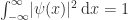$\psi(x)$ does not diverge at the edges of x. If it diverges, it disobeys the condition of square-integrability: $\int_{-\infty}^\infty\!|\psi(x)|^2\,\mathrm{d}x = 1$ and we deal with the physical falseness.

So here’s what we do: we run value of particle’s energy E from 0 to some value, say Vo, and calculate $\psi(x)$ for each E. Value of $\psi(x)$ (at the far outside of the finite well – $\psi(b)$ where b>>L), is put into the separate list whose roots (places where it crosses zero) are to be found. Only those energies E for which $\psi(b)$ is zero are taken in consideration and represent valid state of the particle. Here we see first of many weird things happening in the quantum world – particle can not have any value for kinetic energy, only some of discrete numbers.

Equation solving code

As said earlier, to solve the differential equation we use scipy.integrate.odeint() routine. To properly work with it, we need to rewrite the Schrödinger equation in state-space representation, where first state is $\dot{\psi}$ and second state $\ddot{\psi}$ . Since the odeint() works stepwise, it will take states from the previous step in each computation. The state-space function will finally look like this:

def SE(psi, x):
    """
    Returns derivatives for the 1D schrodinger eq.
    Requires global value E to be set somewhere. State0 is
    first derivative of the wave function psi, and state1 is
    its second derivative.
    """
    state0 = psi[1]
    state1 = 2.0*(V(x) - E)*psi[0]
    return array([state0, state1])

(Note: I’ve put m so that $\hbar^2/m = 1$ , just for simplicity). This function prepares state-space only. Following function does the real job, calls the state-space function and calculates the wave function $\psi(x)$ for a given energy E. It also returns value of $\psi(x)$ at the location x=b to test divergence.

def Wave_function(energy):
    """
    Calculates wave function psi for the given value
    of energy E and returns value at point b
    """
    global psi
    global E
    E = energy
    psi = odeint(SE, psi0, x)
    return psi[-1,0]

Of course, for the first step there is no previous step – that’s why we introduce variable $\psi_0$ , which holds initial conditions: $\psi(0) = 1$ and $\dot{\psi}(0) = 0$

Finding allowed states

Once we have the values of $\psi(b)$ for a range of energies we need to distinguish those states where $\psi(x)$ diverges. This is done using the Brent method to find a zero of the function f on the sign changing interval [a , b]. The method is available as a Python’s routine scipy.optimize.brentq(). For an array of energies e we will check the sign of the $\psi(b)$ . When the sign changes, it means that $\psi(b)$ crosses zero point and now we can call brentq() to find the exact zero-point. The function is embedded as follows:

def find_all_zeroes(x,y):
    """
    Gives all zeroes in y = f(x)
    """
    all_zeroes = []
    s = sign(y)
    for i in range(len(y)-1):
        if s[i]+s[i+1] == 0:
            zero = brentq(Wave_function, x[i], x[i+1])
            all_zeroes.append(zero)
    return all_zeroes

The function will return an array all_zeroes which contains all zero points of the $\psi(b)$ . How nicely the function works, you can see on this image:

Allowed energies for which $\psi(b)$ converges

In this example, I put V₀ to 20, L to 1, and m so that $\hbar^2/m = 1$ . We obtain only 4 four allowed bound states with energies 0.92, 3.65, 8.09, and 14.

Images, yaaay!

Now there’s a little trick. You remember that fantastic little function which solves differential equations, odeint(), needs some initial conditions to work, right?. These are the values of $\psi(x)$ at x=0. What we get from it is the function $\psi(x)$ only right from 0! What happens on the left side? It depends on how we set the initial conditions. For if we chose $\psi(0) = 1$ and $\dot{\psi}(0) = 0$ we get something called symmetrical case, so left side is just mirrored right side. But if we reverse initial conditions so that $\psi(0) = 0$ and $\dot{\psi}(0) = 1$ , we get antisymmetric case. Why is that so? I’ll tell you just that symmetrical states correspond to the cosine based functions, while antisymmetric correspond to the sine based functions. More about it will come a bit later.

Let’s see how the states of $\psi(x)$ look like. For the symmetrical case ( $\psi(0) = 1$ , $\dot{\psi}(0) = 0$ ):

Allowed energies for the symmetrical states

And for the antisymmetrical case ( $\psi(0) = 0$ , $\dot{\psi}(0) = 1$ ):

Allowed energies for the antisymmetrical states

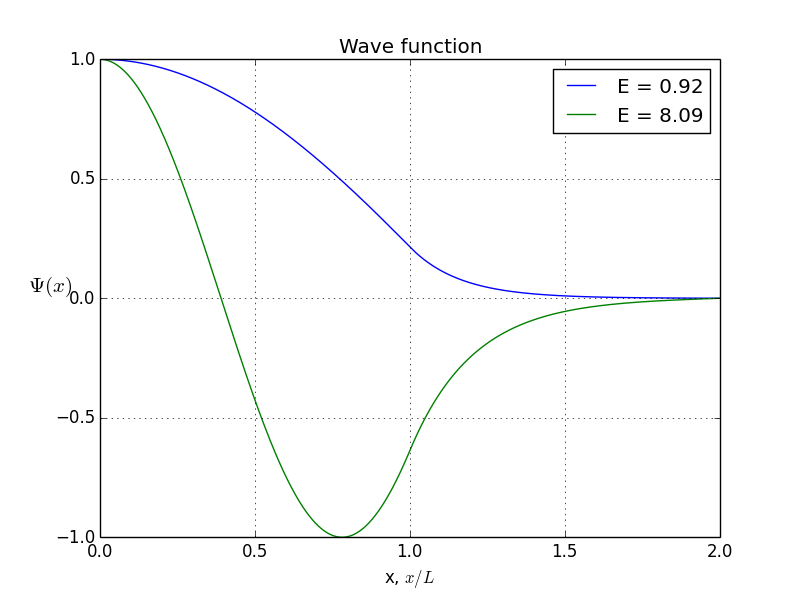
This is nice and correct way to solve the problem of the finite square well. But, I don’t like this boring pictures, so I decided to cheat a little bit :). You see, the odeint() requires the initial conditions at x = 0, assuming x goes from 0 to b. But what if I give it values -b < x< b? Normally, we expect $\psi(-b)$ to be o. But if we put initial conditions to be zero, we won’t get any non-zero result. That’s how the odeint() works, I can not prevent it. So here is where I cheat: I put x to be from -b to b, but initial conditions are not zero. Instead, they are some arbitrarily small value. Of course, odeint() will mess up values, but, interestingly, the shape of the function $\psi(x)$ will stay correct! Additionally, it will calculate both symmetrical and antisymmetrical states. Great!

So, let’s do it again. Energies of allowed states are already calculated, it’s the first graph you see in this article. Bound states are here, presented in symmetrical and antisymmetrical case:

As said earlier, values are messed up, since the integral of $\psi(x)$ squared is not 1. But it doesn’t matter cause $\psi(x)$ is normalized anyway later. Few things about these states.

Particle exists only in discrete states and is associated with the corresponding energy in each state. The states are orthonormal. One state can not be represented as a linear combination of other states. So, the particle can not be in the state which is not representable as a combination of given states.
Probability of finding particle in space is integral of $|\psi(x)|^2$ . We see that in the first state (ground state) most likely to find the particle is in the center of the well. But if you give the particle a bit of energy and it jumps into the second state (excited state) you will find it most likely between center and edges.
What happens with the particle behind the walls of the well? We see that $\psi(x)$ is not zero left from -L and right from L. It means that there is a non-zero probability of finding a particle outside the well! Remember the analogy with the car between the mountains? It would mean that car has somehow ended behind the mountain although it can not climb it. The phenomenon is called quantum tunnelling and it may seem crazy in case of a car and a mountain, but it is quite common and normal thing in subatomic particles.

Is all this right?

Did I do something wrong? Who guarantees that my functions odeint() and brentq() are used properly? Are these solutions of Schrödinger equation correct? To check it, I run a numerical computation of analytical model, provided in “Introduction to Quantum Mechanics” by D. Griffiths, page 62. In that model, we need to find solution of the equation $\tan(z) = \sqrt{(z_0/z)^2-1}$ where $z = \dfrac{\sqrt{(2mE)}L}{\hbar}$ and $z_0 = \dfrac{\sqrt{(2mV_0)}L}{\hbar}$ . This will give us energies of allowed symmetrical states. For antisymmetrical states we should use $-\cot(z) = \sqrt{(z_0/z)^2-1}$ . Python method that does the job is presented here:

def find_analytic_energies(en):
    """
    Calculates Energy values for the finite square well using analytical
    model (Griffiths, Introduction to Quantum Mechanics, page 62.)
    """
    z = sqrt(2*en)
    z0 = sqrt(2*Vo)
    z_zeroes = []
    f_sym = lambda z: tan(z)-sqrt((z0/z)**2-1)      # Formula 2.138, symmetrical case
    f_asym = lambda z: -1/tan(z)-sqrt((z0/z)**2-1)  # Formula 2.138, antisymmetrical case

    # first find the zeroes for the symmetrical case
    s = sign(f_sym(z))
    for i in range(len(s)-1):   # find zeroes of this crazy function
       if s[i]+s[i+1] == 0:
           zero = brentq(f_sym, z[i], z[i+1])
           z_zeroes.append(zero)
    print "Energies from the analytical model are: "
    print "Symmetrical case)"
    for i in range(0, len(z_zeroes),2):   # discard z=(2n-1)pi/2 solutions cause that's where tan(z) is discontinuous
        print "%.4f" %(z_zeroes[i]**2/2)
    # Now for the asymmetrical
    z_zeroes = []
    s = sign(f_asym(z))
    for i in range(len(s)-1):   # find zeroes of this crazy function
       if s[i]+s[i+1] == 0:
           zero = brentq(f_asym, z[i], z[i+1])
           z_zeroes.append(zero)
    print "(Antisymmetrical case)"
    for i in range(0, len(z_zeroes),2):   # discard z=npi solutions cause that's where cot(z) is discontinuous
        print "%.4f" %(z_zeroes[i]**2/2)

As a result, I get output in Python console:

 Energies from the analyitical model are:
 (Symmetrical case)
 0.9179
 8.0922
 19.9726
 (Antisymmetrical case)
 3.6462
 14.0022

and that corresponds completely to programs computation. We can be sure that program works for as long as E is smaller than $V_0$ , and $V_0$ is not unreasonablly large. Finally, the source code for the whole program is here:

# -*- coding: utf-8 -*-
"""
Created on Mon Sep 03 21:02:59 2014

@author: Pero

1D Schrödinger Equation in a finite square well.

Program calculates bound states and energies for a finite potential well. It will find eigenvalues
in a given range of energies and plot wave function for each state.

For a given energy vector e, program will calculate 1D wave function using the Schrödinger equation
in a finite square well defined by the potential V(x). If the wave function diverges on x-axis, the
energy e represents an unstable state and will be discarded. If the wave function converges on x-axis,
energy e is taken as an eigenvalue of the Hamiltonian (i.e. it is alowed energy and wave function
represents allowed state). 

Program uses differential equation solver &amp;amp;amp;quot;odeint&amp;amp;amp;quot; to calculate Sch. equation and optimization
tool &amp;amp;amp;quot;brentq&amp;amp;amp;quot; to find the root of the function. Both tools are included in the Scipy module.
The following functions are provided:

    - V(x) is a potential function of the square well. For a given x it returns the value of the potential
    - SE(psi, x) creates the state vector for a Schrödinger differential equation. Arguments are:
        psi - previous state of the wave function
        x - the x-axis
    - Wave_function(energy) calculates wave function using SE and &amp;amp;amp;quot;odeint&amp;amp;amp;quot;. It returns the wave-function
        at the value b far outside of the square well, so we can estimate convergence of the wave function.
    - find_all_zeroes(x,y) finds the x values where y(x) = 0 using &amp;amp;amp;quot;brentq&amp;amp;amp;quot; tool.    

Values of m and L are taken so that h-bar^2/m*L^2 is 1.

v2 adds feature of computational solution of analytical model from the usual textbooks. As a result,
energies computed by the program are printed and compared with those gained by the previous program.
"""
from pylab import *
from scipy.integrate import odeint
from scipy.optimize import brentq

def V(x):
    """
    Potential function in the finite square well. Width is L and value is global variable Vo
    """
    L = 1
    if abs(x) > L:
        return 0
    else:
        return Vo

def SE(psi, x):
    """
    Returns derivatives for the 1D schrodinger eq.
    Requires global value E to be set somewhere. State0 is first derivative of the
    wave function psi, and state1 is its second derivative.
    """
    state0 = psi[1]
    state1 = 2.0*(V(x) - E)*psi[0]
    return array([state0, state1])

def Wave_function(energy):
    """
    Calculates wave function psi for the given value
    of energy E and returns value at point b
    """
    global psi
    global E
    E = energy
    psi = odeint(SE, psi0, x)
    return psi[-1,0]

def find_all_zeroes(x,y):
    """
    Gives all zeroes in y = Psi(x)
    """
    all_zeroes = []
    s = sign(y)
    for i in range(len(y)-1):
        if s[i]+s[i+1] == 0:
            zero = brentq(Wave_function, x[i], x[i+1])
            all_zeroes.append(zero)
    return all_zeroes

def find_analytic_energies(en):
    """
    Calculates Energy values for the finite square well using analytical
    model (Griffiths, Introduction to Quantum Mechanics, 1st edition, page 62.)
    """
    z = sqrt(2*en)
    z0 = sqrt(2*Vo)
    z_zeroes = []
    f_sym = lambda z: tan(z)-sqrt((z0/z)**2-1)      # Formula 2.138, symmetrical case
    f_asym = lambda z: -1/tan(z)-sqrt((z0/z)**2-1)  # Formula 2.138, antisymmetrical case

    # first find the zeroes for the symmetrical case
    s = sign(f_sym(z))
    for i in range(len(s)-1):   # find zeroes of this crazy function
       if s[i]+s[i+1] == 0:
           zero = brentq(f_sym, z[i], z[i+1])
           z_zeroes.append(zero)
    print "Energies from the analyitical model are: "
    print "Symmetrical case)"
    for i in range(0, len(z_zeroes),2):   # discard z=(2n-1)pi/2 solutions cause that's where tan(z) is discontinous
        print "%.4f" %(z_zeroes[i]**2/2)
    # Now for the asymmetrical
    z_zeroes = []
    s = sign(f_asym(z))
    for i in range(len(s)-1):   # find zeroes of this crazy function
       if s[i]+s[i+1] == 0:
           zero = brentq(f_asym, z[i], z[i+1])
           z_zeroes.append(zero)
    print "(Antisymmetrical case)"
    for i in range(0, len(z_zeroes),2):   # discard z=npi solutions cause that's where ctg(z) is discontinous
        print "%.4f" %(z_zeroes[i]**2/2)

N = 1000                  # number of points to take
psi = np.zeros([N,2])     # Wave function values and its derivative (psi and psi')
psi0 = array([0,1])   # Wave function initial states
Vo = 20
E = 0.0                   # global variable Energy  needed for Sch.Eq, changed in function "Wave function"
b = 2                     # point outside of well where we need to check if the function diverges
x = linspace(-b, b, N)    # x-axis

def main():
    # main program        

    en = linspace(0, Vo, 100)   # vector of energies where we look for the stable states

    psi_b = []      # vector of wave function at x = b for all of the energies in en
    for e1 in en:
        psi_b.append(Wave_function(e1))     # for each energy e1 find the the psi(x) at x = b
    E_zeroes = find_all_zeroes(en, psi_b)   # now find the energies where psi(b) = 0 

    # Print energies for the bound states
    print "Energies for the bound states are: "
    for E in E_zeroes:
        print "%.2f" %E
    # Print energies of each bound state from the analytical model
    find_analytic_energies(en)   

    # Plot wave function values at b vs energy vector
    figure()
    plot(en/Vo,psi_b)
    title('Values of the $\Psi(b)$ vs. Energy')
    xlabel('Energy, $E/V_0$')
    ylabel('$\Psi(x = b)$', rotation='horizontal')
    for E in E_zeroes:
        plot(E/Vo, [0], 'go')
        annotate("E = %.2f"%E, xy = (E/Vo, 0), xytext=(E/Vo, 30))
    grid()

    # Plot the wavefunctions for first 4 eigenstates
    figure(2)
    for E in E_zeroes[0:4]:
        Wave_function(E)
        plot(x, psi[:,0], label="E = %.2f"%E)
    legend(loc="upper right")
    title('Wave function')
    xlabel('x, $x/L$')
    ylabel('$\Psi(x)$', rotation='horizontal', fontsize = 15)
    grid()

if __name__ == "__main__":
    main()

32 thoughts on “Quantum Mechanics with the Python”

8in8 says:

September 5, 2014 at 3:48 am

Thank you
Blog fantastic
Good luck
……………….
http://www.8ii.in

Reply
1. Pero says:
  
  September 5, 2014 at 9:48 am
  
  Thanks, I’m glad that you liked it!
  
  Reply
Jean-Luc Orgiazzi says:

September 5, 2014 at 3:54 am

Next, you can play with Qutip (http://qutip.org/).
Cheers!

Reply
1. Pero says:
  
  September 5, 2014 at 9:47 am
  
  Wow, this sounds pretty cool! Thanks
  
  Reply
presveva says:

September 5, 2014 at 10:09 am

this post is now in my resume at the section “reading” 🙂

Reply
Anandaram Mandyam says:

September 7, 2014 at 10:07 am

I just executed your 1DSE for finite Sq Well and it gave two nice plots.
The 2nd plot titled “wave function” should be renamed “probability density, \Psi(x)^2”.
Si I added a 3rd plot for just the “wave function,\Psi(x)” by omitting the squaring:
The two plot codes are listed below:
# Plot the wavefunctions for first 4 eigenstates
figure(2)
for E in E_zeroes[0:4]:
Wave_function(E)
plot(x, psi[:,0], label=”E = %.3f”%E)
legend(loc=”upper right”, frameon=False)
title(‘Wave function, $\Psi(x)$’)
xlabel(r’x, $x/L$’)
ylabel(r’$\Psi(x)$’, rotation=’horizontal’, fontsize = 15)
grid()

# Plot the probability densities for first 4 eigenstates
figure(3)
for E in E_zeroes[0:4]:
Wave_function(E)
plot(x, psi[:,0]**2, label=”E = %.3f”%E)
#xlim(())
ylim((-1000,35000))
legend(loc=”upper right”, frameon=False)
title(‘Probabability density, $\Psi(x)^2$’)
xlabel(r’x, $x/L$’)
ylabel(r’$\Psi(x)^2$’, rotation=’horizontal’, fontsize = 15)
grid()
———————————————————————————————–
Overall a nice effoet. Keep going.

Reply
1. Pero says:
  
  September 13, 2014 at 1:47 pm
  
  Thanks for the feedback! You’re right, I forgot that I changed the code before updating post!
  
  Reply
dguitarbite says:

September 10, 2014 at 7:59 pm

Reblogged this on Rocker/Hacker and commented:
Wow, I wanna revise Quantum Mechanics now!

Reply
1. Pero says:
  
  September 13, 2014 at 1:42 pm
  
  Thanks, I’m glad you like it. Keep on rockin’!
  
  Reply
Anandaram Mandyam says:

September 14, 2014 at 11:16 am

Hi: The energy level of 19.9726 given by the analytical model is not detected
by the brentq() procedure. I failed to get it even with setting b = 3 and Nsteps to 3000.
What could be the reason?

Reply
1. Pero says:
  
  September 14, 2014 at 2:03 pm
  
  Thanks for the reply, Anandaram, I am happy to see that my post interests you so much! Regarding your question, I tested the program and this is my conclusion: brentq() fails to find last energy level because odeint() doesn’t give solution which drops so fast at b! This is because of relatively small potential V0 – the smaller V0, the wave function lives longer outside the well, and program can not find its exact zero-value. Solution to this problem? Increase V0 or b! Than the numerical values of energies will give you exact energies from analytic model!
  
  Cheers!
  
  Reply
Anandaram Mandyam says:

September 19, 2014 at 3:27 pm

Thanks for your advice. The problem rarely recurs when Vo is increased keeping b = 3.
I found the plotted curves at their best when I set psi0 = [1.0e-15, 1.0e-5]. I applied your
program to the case of Vo = Inf. It didn’t work. Then I set b = L = 1 itself with Vo = 50(say).
Expected results came along nicely. The wavefunction plot is quite like your plot above but
truncated between -1 and 1. This I think mimics Inf potential result. Hope this interests
your readers.
Anandaram

Reply
taquan soho says:

November 4, 2014 at 12:00 pm

How to extend this to a 2D particle-in-a-box ?

Reply
1. Pero says:
  
  November 10, 2014 at 7:43 pm
  
  Hi,
  I guess nice try would be making a matrix in x,y coordinates and solve the schroedinger equation in odeint() with two variables. I am only not sure wheather the Python (odeint) supports such an extravaganze
  
  Reply
arnaldo armida says:

December 7, 2014 at 9:02 am

Hi,
sorry for my question..I’m a beginner….so….forgive me:)
running the software I get the equation solution in the terminal but not the plots…I’m using qutip ..
Energies for the bound states are:
Shroedinger_1.py:90: RuntimeWarning: divide by zero encountered in divide
f_sym = lambda z: tan(z)-sqrt((z0/z)**2-1) # Formula 2.138, symmetrical case
Energies from the analyitical model are:
Symmetrical case)
0.9179
8.0922
19.9726
Shroedinger_1.py:91: RuntimeWarning: divide by zero encountered in divide
f_asym = lambda z: -1/tan(z)-sqrt((z0/z)**2-1) # Formula 2.138, antisymmetrical case
(Antisymmetrical case)
3.6462
14.0022
/usr/lib/pymodules/python2.7/matplotlib/axes.py:4747: UserWarning: No labeled objects found. Use label=’…’ kwarg on individual plots.
warnings.warn(“No labeled objects found. ”

——-
Where is my mistake?
Thanks a lot for your help
Arnaldo

Reply
1. Pero says:
  
  December 8, 2014 at 7:45 pm
  
  what do you mean, you’re using qtip? If you run my code on the python supporting platform, there should be no error messages.
  
  Reply
  1. Arnaldo Armida says:
    
    December 9, 2014 at 3:32 pm
    
    Thanks for your reply…
    I mean that I have used the Qutip (http://qutip.org/)platform….but it doesn’t matter..
    Using the platform you have used I get the numeric solutions but not the plots.
    It’s surely my fault but I do not know where I made mistake!
    Sorry to disturb you.
    Regards.
    Arnaldo
    
    Reply
2. Pero says:
  
  December 12, 2014 at 9:29 am
  
  sorry, for some reason I can not answer your latest post, so I’ll write here. Are you sure that all your modules are installed in proper version? Maybe you’re using Python 3?
  
  Reply
  1. esperia says:
    
    December 12, 2014 at 11:41 am
    
    Hi,
    thanks for your reply and thanks for your patience!
    I’m using python 2.7 as you can see from the following:Last login: Thu Dec 11 09:37:03 on ttys002
    MacArnaldo:~ arnaldoarmida$ python
    Python 2.7.9rc1 (v2.7.9rc1:40eada278702, Nov 25 2014, 17:25:50)
    [GCC 4.2.1 (Apple Inc. build 5666) (dot 3)] on darwin
    Type “help”, “copyright”, “credits” or “license” for more information.
    >>> from pylab import *
    >>> from scipy.integrate import odeint
    >>> from scipy.optimize import brentq
    >>>
    The system is MAC..but the same I have in Linus Ubuntu..
    AS you can see I have put in a terminal the calls to the libraries and I do not get errors…..
    I’m really sorry…
    You can be so kind to tell me what python have you used and all the libraries you have used?..it can solve the problem since I will follow step by step everything.
    Waiting for your kind reply.
    Arnaldo
    
    Reply
  2. Arnaldo Armida says:
    
    December 12, 2014 at 11:43 am
    
    Hi,
    thanks for your reply and thanks for your patience!
    I’m using python 2.7 as you can see from the following:Last login: Thu Dec 11 09:37:03 on ttys002
    MacArnaldo:~ arnaldoarmida$ python
    Python 2.7.9rc1 (v2.7.9rc1:40eada278702, Nov 25 2014, 17:25:50)
    [GCC 4.2.1 (Apple Inc. build 5666) (dot 3)] on darwin
    Type “help”, “copyright”, “credits” or “license” for more information.
    >>> from pylab import *
    >>> from scipy.integrate import odeint
    >>> from scipy.optimize import brentq
    >>>
    The system is MAC..but the same I have in Linus Ubuntu..
    AS you can see I have put in a terminal the calls to the libraries and I do not get errors…..
    I’m really sorry…
    You can be so kind to tell me what python have you used and all the libraries you have used?..it can solve the problem since I will follow step by step everything.
    Waiting for your kind reply.
    Arnaldo
    
    Reply
3. Pero says:
  
  December 12, 2014 at 11:54 am
  
  everything seems fine, judging from your latest post. I used also Python 2.7 in Spyder software tool on Win 7. Sorry, but I honestly have no idea for what may cause your problems. Try to run the program on some windows computer. If it works it must have been some Mac/Linux incopatibility issue.
  
  Reply
4. emanuelfontelles says:
  
  January 20, 2015 at 9:55 pm
  
  I had the same mistake, are you corrected?
  
  Reply
  1. arnaldo armida says:
    
    January 21, 2015 at 8:30 am
    
    Hi There, yes..
    
    I have installed the ” spyder” suite..and finallyy I have got the graphs..https://pypi.python.org/pypi/spyder
    Try this..and i hope it will help.
    Arnaldo
    
    Reply
Sachin says:

December 7, 2014 at 1:44 pm

Hello all,
I am reading such posts of animation of quantum mechanics equations using python. I want to learn it. May I know the minimum requirement of tools. Mathematics, python relation files etc and their combination to use.
I have basic python only. and I know a bit of that only. Please suggest stepwise and I will try to learn.
Thanks
Sachin
sacheein@gmail.com

Reply
1. Pero says:
  
  December 8, 2014 at 7:43 pm
  
  Hello Sachin. To learn Python I used many online resources and tutorials. There are multiple blogs and online courses that teach you, this one in.e. http://openedx.seas.gwu.edu/courses/GW/MAE6286/2014_fall/info I started with Python many years ago with simple book “Python for dummies”.
  To learn QM on very very basic level I recommend “Introduction to quantum mechanics” by D. Griffiths. Under assumption, of course, that you are familiar with the first-year mathematics (calculus, linear algebra, vectors etc)
  
  Reply
quantuman says:

December 10, 2014 at 6:21 pm

hi,

I’m a new user of Python, and i’m wondering if I’m able to make a program for quantum dots without the “fenics”, and if there’s any references it will be helpful

Reply
Pingback: QM with Python – swing on the quantum harmonic oscillator | HELENTRONICA
Alexandre says:

June 9, 2015 at 3:57 pm

I found a mistake in your code, the potential is inverted, you have a wall instead of a well.

Reply
1. Pero says:
  
  June 10, 2015 at 1:03 pm
  
  Though I disagree, thank you for your opinion. Could you point out more precisely what error did you find?
  
  Reply
  1. Nishant says:
    
    August 8, 2016 at 9:57 pm
    
    The error he found was:
    
    def V(x):
    “””
    Potential function in the finite square well. Width is L and value is global variable Vo
    “””
    L = 1
    if abs(x) > L:
    return 0
    else:
    return Vo
    
    This is what you have in the code above, but if you look at it carefully, it shows that its a wall. When I run the code as is, I do not get any bound solutions numerically. If I switch 0 and Vo, then I get all the same plots you have shown in the blog post.
    
    Reply
    1. The Relative Luminosity (@stjertmeis) says:
      
      July 9, 2020 at 12:00 am
      
      I agree with Alexandre and Nishant. I did not get energy for bound state solutions with the current code. Alternative to what Nishant used, changing “abs(x)<L" to get 0 also works, which is the condition for finite well.
      
      Reply
uni-fiz says:

September 12, 2015 at 8:18 pm

How to calculate energy states and w.functions in multilayer quantum wells?

Reply