QM with Python – swing on the quantum harmonic oscillator

Introduction

(This post continues on my older post on using Python in solving simple quantum mechanics problems)

A completely simple everyday example of harmonic motion on a pendulum — A completely simple everyday example of a harmonic motion on a pendulum

You have heard of harmonic oscillator in physics classroom. It is a simple mathematical tool to describe some kind of repetitive motion, either it is pendulum, a kid on a sway, a kid on a spring or something else. As long as it goes back and forth in periodical way, it’s a harmonic oscillator. Usual way of solving HO motion is classic Newton’s mechanics. We’d start with the basic equations of motion, something like $\ddot{x}+\omega^2 x = 0$ , where x is the spatial variable (it can be displacement in spring system, but also an angle for the pendulum case), and $\omega$ is a frequency of the oscillation. Solution is always some combination of sine and cosine function. The very same problem can be solved using quantum mechanics, i.e. Schrödinger equation. Solution in that case is weird, something completely contrary to our everyday experiences, but perfectly suitable for microcosmos of atoms and elementary particles. This kind of craziness I’ll try to present with help of programming language Python.

Potential function

We start again with her majesty, Schrödinger equation:

So, to make long story short: $\psi(x)$ is a wave function associated with our particle – it has no meaning per se, but $\left|\psi(x)\right|^2$ is a probability of finding the particle at the place x. Solving the equation will tell us this probability. Regarding other symbols, m is a mass of the particle, E is its energy, $\hbar$ is reduced Planck’s constant and 2 is just a number 2. V(x) is something interesting – it is the potential function. What does it mean? Potential is something that controls the particle. We are everyday controlled by the gravitational potential of our Earth – we all have a tendency to go down, we fall when standing free in the air. The higher we are, our potential energy is bigger, because the potential V(x) is higher. Everything has a tendency to move to the lower potential, whether it is body in gravitational field, charged particle in electrical field or something third. No wonder, because the gradient of the potential, $\nabla \cdot V(x)$ , is nothing more than a force, pulling the body towards the lower potential energy state.

Approximation of any ugly potential function as a pretty parabolic HO potential with a puppy. — Approximation of any ugly potential function with a pretty parabolic HO potential with a puppy (from the Griffith’s *Introduction to QM*).

Potential function is a space dependent function. It varies with x, and it can vary in many different ways, like on the image above. It may be very hard to describe it mathematically in a nice way. But we don’t care for all x-s in the world – we are interested in what happens in some constrained area, say, surrounding of this gap at $x_0$ , which we will call local minimum. This is obviously the place where the force will pull the body to. If we want to approximate V(x) at this point we’ll do it by expanding Taylor’s series:

$V(x) = V(x_0) + \frac{dV}{dx}(x-x_0) + \frac{1}{2!}\frac{d^2V}{dx^2}(x-x_0)^2 +\frac{1}{3!}\frac{d^3V}{dx^3}(x-x_0)^3 + \ldots$

Now, since $x_0$ is local minimum, we know that first derivative of V(x) will be zero. Second derivative will remain, but any derivative of higher order will vanish. The first term, $V(x_0)$ is constant and independent of x and can be ignored. Finally, we can shift our x-axis to the point where $x_0$ is 0. Our potential function now looks like this: $V(x) = \frac{1}{2} k x^2$ , where k is some constant of proportionality. Interestingly, potential energy of the body on the spring is exactly $\frac{1}{2} k x^2$ if k is the spring constant.

Going the Python way

In my older post, I used Python to solve some simple problems of quantum mechanics. The very same applies here. Firstly, I’ll define potential function, V(x). For every point x, the function checks whether x is within the region of HO. If it is, output value is $\frac{1}{2} k x^2$ . Otherwise, output is some constant value.

def V(x):
    """
    Potential function in the Harmonic oscillator. Returns V = 0.5 k x^2 if |x|&lt;L and 0.5*k*L^2 otherwise
    """    
    if abs(x)<L:
        return 0.5*k*x**2
    else:
        return 0.5*k*L**2

Equation solver

Schrödinger’s equation is 2nd order differential equation and nobody with the clear mind wants to solve it by hand. Instead, normal people use Python embedded numerical solver odeint() from scipy.integrate package. We’ll first rewrite this perverse equation as a system of two 1st order diff. equations by introducing a new variable $bunny := \dot{\psi}$ , so that the system becomes:

$\dot{\psi} = bunny$

$\dot{bunny} = \frac{2m}{\hbar^2} ( V(x) - E ) \psi$

Left sides of the equations, we will call them states, as they are representing the state space of the system. The odeint() will solve two of them at the same time and put the solutions in a 2×length(x) – sized array called psi (global variable here). All this is done in the function Wave_function(). The other function, SE(), prepares the derivatives from the given wave function psi. As always when solving diff. equations, we need to specify initial conditions which will be in a 2-element array psi_init. These will be very low, cause we expect the wave function to vanish at the position outside of the HO.

def SE(psi, x):
    """
    Returns derivatives for the 1D schrodinger eq.
    Requires global value E to be set somewhere. State0 is
    first derivative of the wave function psi, and state1 is
    its second derivative.
    """
    state0 = psi[1]
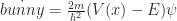
    state1 = 2.0*(V(x) - E)*psi[0]
    return array([state0, state1])

def Wave_function(energy):
    """
    Calculates wave function psi for the given value
    of energy E and returns value at point b
    """
    global psi
    global E
    E = energy
    psi = odeint(SE, psi_init, x)
    return psi[-1,0]

Finding alowed states

The problem is – upper program will work almost all the time :). We can get infinitely many solutions. And that’s bad. cause not all of them are meaningful. We need to find only those solutions where wave function $\psi(x)$ converges at the edges of x. If it doesn’t, it means that particle is not localized – it appears to be everywhere with the total probability more than 1! This is physically false. So here’s what we do: we run value of particle’s energy E from 0 to some value, say Emax, and calculate $\psi(x)$ for each E. Value of $\psi(x)$ outside of the HO is put into the separate psi_end list whose roots (places where it crosses zero) are to be found. Only those energies E for which wave function is zero are taken into consideration and they represent the valid state of the particle. Here we see one of many weird things happening in the quantum world – particle can not have any value for its energy, only some of discrete numbers.

Once we have the values of psi_end for a range of energies we need to distinguish those states where wave function diverges. This is done using the Brent method to find a zero of the function f on the sign changing interval [x , x+dx]. The method is available as a Python’s routine scipy.optimize.brentq(). For an array of energies E we will check the sign of the psi_end. When the sign changes, it means that psi_end crosses zero and now we can call brentq() to find the exact zero-point. The function is embedded as follows:

def find_all_zeroes(x,y):
    """
    Gives all zeroes in y = f(x)
    """
    all_zeroes = []
    s = sign(y)
    for i in range(len(y)-1):
        if s[i]+s[i+1] == 0:
            zero = brentq(Wave_function, x[i], x[i+1])
            all_zeroes.append(zero)
    return all_zeroes

Results and “is this correct?”

To make life easier, I put values for $k, \hbar \text{ and } m$ to be 100, 1 and 1, respectively. First figure shows how psi_end varies for different energies. The program found those energies E for which psi converges outside of the HO. These correspond to so-called eigenstates of the harmonic oscillator. How many of these are there anyway? Actually, theory of the quantum HO is simple: for n-th eigenstate of HO, energy will be $E = \hbar \omega(n+0.5)$ . Knowing that $\omega = \sqrt{k/m}$ , we can expect energies of 5, 15, 25, 35 and 45. Triumphantly, they are exactly what the program has found!

Allowed energies for the quantum harmonic oscillator (only lowest 4)

Now that we have required energies, we can’t wait to see how the particle will behave. Next plot shows the probability density function for the first 4 eigenstates. It looks pretty weird, huh? Let’s check what classical physics tells us. All the time energy of the body is constant and it is a sum of its kinetic and potential energy. At the balance point, the potential energy is zero meaning that kinetic energy is maximum. So the highest speed particle can have is when it is passing through the balance point. Logically, there is the least probability of finding a particle there. Vis-a-vis to that, at the edges of the oscillator particle has no kinetic energy at all, therefore speed is zero, therefore there is the most chance of finding the particle there. But check the plot again. It doesn’t work that way for quantum physics. Here, for the lowest energy, probability of finding a particle is the greatest in the middle, at the balance point. Why is that so? How is that possible?!

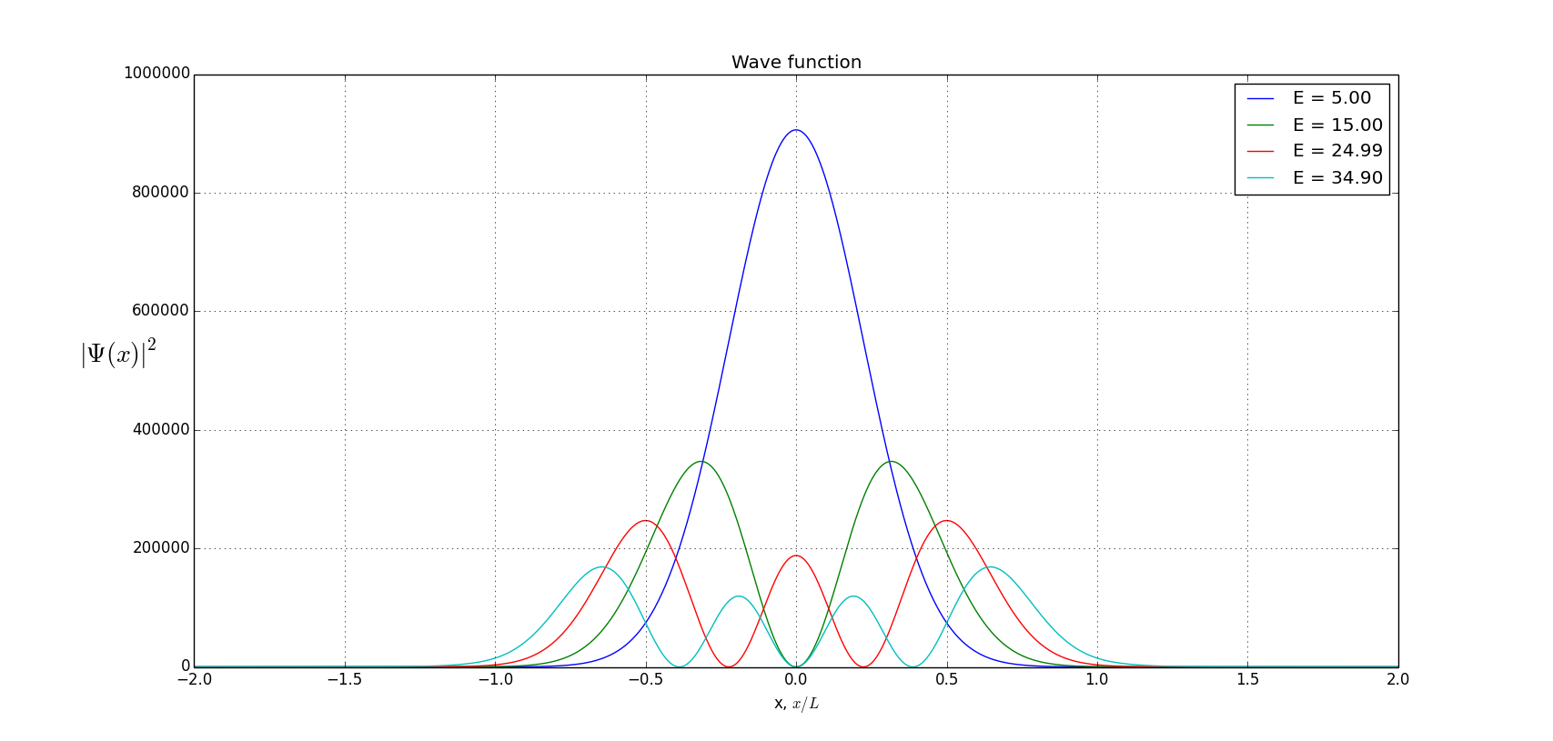
Wave functions for 4 lowest states of quantum harmonic oscillator. Here you see where is the most probable to find a particle with a specific energy.

The truth is – no one knows. There are many different interpretations of quantum physics and no way to prove any of them. It just works that way. If you put an electron at the minimum energy in the oscillating state, you’ll most likely find it in the middle. But the same will not be true if you put a pup on a swing in the oscillating state. How is that so? Shouldn’t the Schrödinger equation work the same for both electron and the puppy?

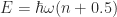
It should and it does. Only difference is that the puppy has a much much greater energy than the electron. Check the expression for the energy above. Since the Planck constant is ridiculously small number, quantum number n has to be insanely big to be adequate for the dog on the swing. Let’s see what happens if we increase n to, say, 50 (actually, I put the mass m = 100. Now I can keep energy vector lower than the maximum potential energy of HO but with better resolution).

Probability density of particle with high quantum number, in e. puppy in the swing

Ha, beautiful! It looks more like what we would expect from the classical mechanics – the probability is lowest in the middle. I find it amazing how such simple program can find such complex functions. But still, there are some peaks and dips along the x-axis. Still not exactly what we would like it to be. But don’t worry, in a world where we and the puppy live, the quantum number is so large and width of the dips is so small that there are no means to measure them. For us, probability density function is a smooth line along the x, just the way we’d expect from the classical physics. And there is a name for this – a correspondence principle. It says that when the quantum number n goes insanely large, quantum mechanics starts to reproduce classical physics. In other words, for the large energies quantum calculations must agree with classical calculations. Correspondence principle is next big thing coming up from quantum mechanics after the energy discreteness and quantum tunneling which I covered in previous post.

Complete Python code for one-dimensional quantum harmonic oscillator can be found here:

# -*- coding: utf-8 -*-
"""
Created on Sun Dec 28 12:02:59 2014

@author: Pero

1D Schrödinger Equation in a harmonic oscillator.

Program calculates bound states and energies for a quantum harmonic oscillator. It will find eigenvalues 
in a given range of energies and plot wave function for each state.

For a given energy vector e, program will calculate 1D wave function using the Schrödinger equation
in the potential V(x). If the wave function diverges on x-axis, the
energy e represents an unstable state and will be discarded. If the wave function converges on x-axis, 
energy e is taken as an eigenvalue of the Hamiltonian (i.e. it is alowed energy and wave function
represents allowed state). 

Program uses differential equation solver &quot;odeint&quot; to calculate Sch. equation and optimization
tool &quot;brentq&quot; to find the root of the function. Both tools are included in the Scipy module.
The following functions are provided:

    - V(x) is a potential function of the HO. For a given x it returns the value of the potential
    - SE(psi, x) creates the state vector for a Schrödinger differential equation. Arguments are:
        psi - previous state of the wave function
        x - the x-axis
    - Wave_function(energy) calculates wave function using SE and &quot;odeint&quot;. It returns the wave-function
        at the value b far outside of the square well, so we can estimate convergence of the wave function.
    - find_all_zeroes(x,y) finds the x values where y(x) = 0 using &quot;brentq&quot; tool.    

Vales of m and L are taken so that h-bar^2/m*L^2 is 1.

v2 adds feature of computational solution of analytical model from the usual textbooks. As a result, 
energies computed by the program are printed and compared with those gained by the previous program.
"""
from pylab import *
from scipy.integrate import odeint
from scipy.optimize import brentq
#import matplotlib as plt

def V(x):
    """
    Potential function in the Harmonic oscillator. Returns V = 0.5 k x^2 if |x|&lt;L and 0.5*k*L^2 otherwise
    """    
    if abs(x)< L:
        return 0.5*k*x**2
    else:
        return 0.5*k*L**2
        
def SE(psi, x):
    """
    Returns derivatives for the 1D schrodinger eq. 
    Requires global value E to be set somewhere. State0 is first derivative of the 
    wave function psi, and state1 is its second derivative.
    """
    state0 = psi[1]
    state1 = (2.0*m/h**2)*(V(x) - E)*psi[0]
    return array([state0, state1])
    
def Wave_function(energy):
    """
    Calculates wave function psi for the given value 
    of energy E and returns value at point b
    """
    global psi
    global E
    E = energy
    psi = odeint(SE, psi_init, x)
    return psi[-1,0]

def find_all_zeroes(x,y):
    """
    Gives all zeroes in y = f(x)
    """
    all_zeroes = []   
    s = sign(y)
    for i in range(len(y)-1):
        if s[i]+s[i+1] == 0:
            zero = brentq(Wave_function, x[i], x[i+1])
            all_zeroes.append(zero)
    return all_zeroes
    

    
def find_analytic_energies(en):
    """ 
    Calculates Energy values for the harmonic oscillator using analytical
    model (Griffiths, Introduction to Quantum Mechanics, page 35.)
    """
    E_max = max(en)
    print 'Allowed energies of HO:'
    i = 0
    while((i+0.5)*h*w < E_max):
        print '%.2f'%((i+0.5)*h*w)
        i+=1
    
    
    
N = 1000                  # number of points to take on x-axis    
psi = np.zeros([N,2])     # Wave function values and its derivative (psi and psi')
psi_init = array([.001,0])# Wave function initial states
E = 0.0                   # global variable Energy  needed for Sch.Eq, changed in function "Wave function"
b = 2                     # point outside of HO where we need to check if the function diverges
x = linspace(-b, b, N)    # x-axis
k = 100                   # spring constant 
m = 1                     # mass of the body
w = sqrt(k/m)             # classical HO frequency 
h = 1                     # normalized Planck constant
L = 1                     # size of the HO
               
def main():    
    # main program        
    
    en = linspace(0, 0.5*k*L**2, 50)   # vector of energies where we look for the stable states
    
    psi_end = []      # vector of wave function at x = b for all of the energies in en
    for e1 in en:
        psi_end.append(Wave_function(e1))     # for each energy e1 find the the psi(x) outside of HO        
        
    E_zeroes = find_all_zeroes(en, psi_end)   # now find the energies where psi(b) = 0 
    
    #Plot wave function values at b vs energy vector
    figure()
    plot(en,psi_end)
    title('Values of the $\Psi(b)$ vs. Energy')
    xlabel('Energy, $E$')
    ylabel('$\Psi(x = b)$', rotation='horizontal')
    for E in E_zeroes:
        plot(E, [0], 'go')
        annotate("E = %.2f" %E, xy = (E, 0), xytext=(E, 5))
    grid()
       
    # Print energies for the found states
    print &quot;Energies for the bound states are: &quot;
    for En in E_zeroes:
        print "%.2f " %En
        
    # Print energies of each bound state from the analytical model
    find_analytic_energies(en)   

    # Plot the wave function for 1st 4 eigenstates
    figure(2)
    for i in range(4):                                                 # For each of 1st 4 allowed energies
        Wave_function(E_zeroes[i])                                     # find the wave function psi(x) 
        plot(x, 100**i*psi[:,0]**2, label="E = %.2f" %E_zeroes[i])      # and plot it scaled for comparison    
    legend(loc="upper right")
    title('Wave function')
    xlabel('x, $x/L$')
    ylabel('$|\Psi(x)|^2$', rotation='horizontal', fontsize = 20)    
    grid()       
    
    # Plot the wave function for the last eigenstate
    figure(3)
    Wave_function(E_zeroes[-1])                                        # Find Wave function for the last allowed energy
    plot(x, psi[:,0]**2, label="E = %.2f" %E_zeroes[-1])    
    legend(loc="upper right")
    title('Wave function')
    xlabel('x, $x/L$')
    ylabel('$|\Psi(x)|^2$', rotation='horizontal', fontsize = 20)    
    grid()    
    
if __name__ == "__main__":
    main()

One thought on “QM with Python – swing on the quantum harmonic oscillator”

Avik says:

April 26, 2022 at 4:02 pm

This is really helpful seriously. So thanks for this kind of work.